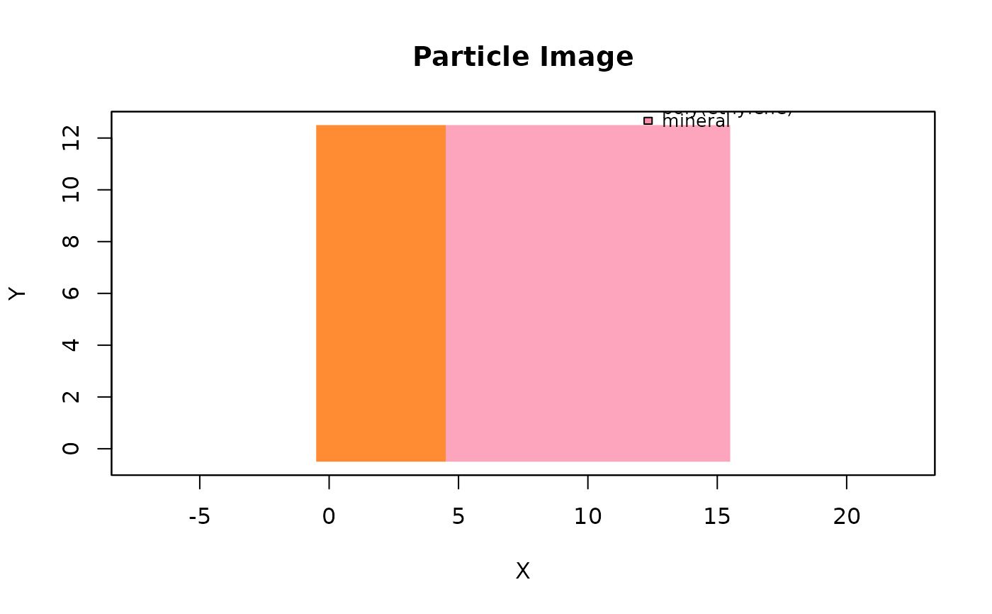
Plot particle maps with base graphics — particle

particle_image() plots particle classifications from an OpenSpecy, Specs, or metadata table. When a visual image is attached with add_visual_image() or supplied directly, particle coordinates are transformed onto the image and drawn as a transparent categorical raster.

Usage

particle_image(
  x,
  material_col = "material_class",
  image = NULL,
  bottom_left = NULL,
  top_right = NULL,
  pixel_length = 1,
  origin = c(0, 0),
  palette = NULL,
  alpha = 0.8,
  labels = FALSE,
  label_col = "feature_id",
  main = "Particle Image",
  xlab = "X",
  ylab = "Y",
  legend = FALSE,
  pch = 15,
  cex = 1,
  ...
)

Arguments

x: an OpenSpecy object, Specs object, or metadata table.
material_col: column containing material or class labels.
image: optional image path, array, raster, raw BMP bytes, or image object. If NULL, an attached visual image is used when available.
bottom_left, top_right: optional map extent in image pixel coordinates.
pixel_length: map pixel length in plotting units when no image overlay is used.
origin: numeric length-2 x/y origin offset when no image overlay is used.
palette: named character vector mapping materials to colors.
alpha: transparency for particle raster cells.
labels: logical; draw feature labels when feature IDs are present? The default is FALSE because particle maps quickly become cluttered.
label_col: column used for labels.
main, xlab, ylab: plot labels.
legend: logical; draw a base graphics legend?
pch, cex: retained for compatibility; particle cells are drawn as a raster.
...: additional arguments passed to plot().

Value

Invisibly returns the plotted metadata table.

Examples

tiny_map <- read_extdata("CA_tiny_map.zip") |> read_any()
tiny_map$metadata$material_class <- ifelse(tiny_map$metadata$x < 5,
                                           "poly(ethylene)", "mineral")
particle_image(tiny_map, legend = TRUE)